Introduction
I use "we" here because writing in first person sounds really weird in this context.
The double inverted pendulum on a cart (DIPC) is a classic example of an underactuated nonlinear system presenting significant challenges in control design. In this project, we design a nonlinear receding-horizon model-predictive controller to perform swing-up and stabilizing control. We then evaluate this controller in a Simulator in the Loop (SITL) environment as well as on a physical system.
Problem Formulation
In this project, we aim to use MPC to stabilize an inverted double pendulum attached to a cart, shown in Figure 1.
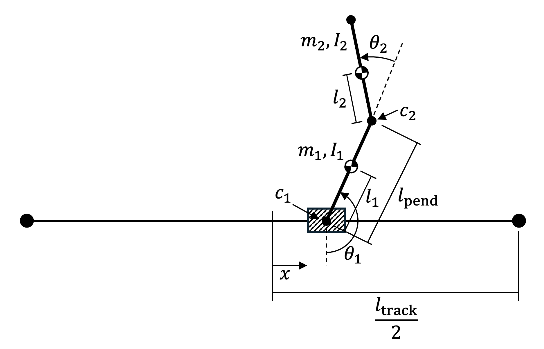
In Figure 1,
In order to design a controller for the system, we must first develop a dynamic model for it. To do so, we calculate the kinetic and potential energies of the system and then apply Lagrange's equations to determine the equations of motion.
Dynamics
We use the method of Lagrange to formulate the system dynamics in the form
The math described here was done using SymPy, a computer algebra system for python. The expressions were then converted to CasADi expressions for fast evaluation, derivatives, and interfacing to optimization engines.
Kinematics
First, we formulate all necessary cartesian positions and velocities from our generalized coordinates
Given this, we can also compute the position of the center of mass of each pendulum:
Taking a time derivative, we can compute the velocities:
Lagrangian
The total translational kinetic energy of the links is then
We can then write these equations in state-space form and incorporate the non-conservative friction forces, which we approximate as viscous friction.
where
In the following sections, our objective will be to use an MPC to stabilize the system about various equilibrium points: the down-up configuration
Controller Design
To design our controller, we first formulate the problem we are trying to solve as a nonlinear constrained infinite time optimal control problem, then approximate this as a receding horizon control problem by designing terminal costs and constraints, which we compute approximately from a linearization and corresponding linear quadratic regulator.
First, our complete discrete nonlinear constrained infinite time optimal conctrol problem is as follows:
where
Receding Horizon Formulation
This full problem is infeasible to solve online, largely because of the infinite sum. To make a problem that is solvable online, we reformulate the problem as a receding horizon problem, limiting the length of a sum to a constant horizon length
again, with the tilde indicating deviation from the reference trajectory. Path tracking will be discussed more in depth in path following; for now it is safe to assume that the reference is simply an equilibrium point
Recursive Feasibility and Stability
To ensure that the above problem is recursively feasible and that our desired equilibrium is Lyapunov stable under the resulting controller, we first linearize the system and compute the discrete LQR controller. We define
to be our linearized system about the equilibrium point
We take
In order to enforce recursive stability, we compute the maximal positive invariant set for the closed-loop linear system
To ensure we meet our recursive feasibility requirements, we need to also ensure that the terminal cost is a Lyapunov function for the system with the simple LQR controller over all of the terminal set
We want to find where the function
This is hard to solve numerically, so we reformulate it as a minimization:
Once we obtain some optimal value
These two terminal constraints - the polytopic constraint from the linear system and this quadratic constraint - do not guarantee recursive feasibility or stability because the linearized model was used to compute the
Terminal Constraint Problems
Unfortunately, the terminal constraint derived above proved to be impractically small. Because this system operates on a very fast timescale, the time horizon for the online MPC controller had to be rather limited to be computationally feasible. This meant that the initially feasible set
Despite the terminal constraint giving much stronger theoretical notions of stability and feasibility, the small feasible set meant that in practice the controller without the terminal constraint was far more robust. This means that ultimately, the terminal constraint had to be discarded.
In order to tackle the more complicated swing-up maneuvers, since we could not rely on the online algorithm to remain feasible or see that far ahead, we solved a full constrained, finite-time optimal control problem offline (ie, batch approach) to generate a trajectory for the controller to track. While tracking a trajectory, the terminal cost is no longer a good approximation for the true cost to go, but computing a more accurate cost to go proved both difficult and uneccessary - the controller performed swing-up well regardless.
Implementation
The controller was implemented using CasADi for automatic differentiation and code generation, IPOPT for solving the nonlinear program, and HSL MA57 for solving the sparse symmetric linear systems needed for IPOPT's newton steps.
We took a direct multiple-shooting (ie, no substitution) approach and used a single step of euler's method to integrate between each timestep. This is an algorithm with known poor performance, but this is okay because the time scales are short and computation time is of utmost importance.
We experimented with many different methods and tools for each of these steps, and those listed above proved the fastest. Other options we tried included:
- NLP solvers: WORHP, SNOPT
- Linear Solvers: MUMPS, MA27, MA97
- integration methods: RK45, IDAS, CVODES, midpoint
With proper warmstarting, we were able to acheive solve times in the neighborhood of 6-8 milliseconds.
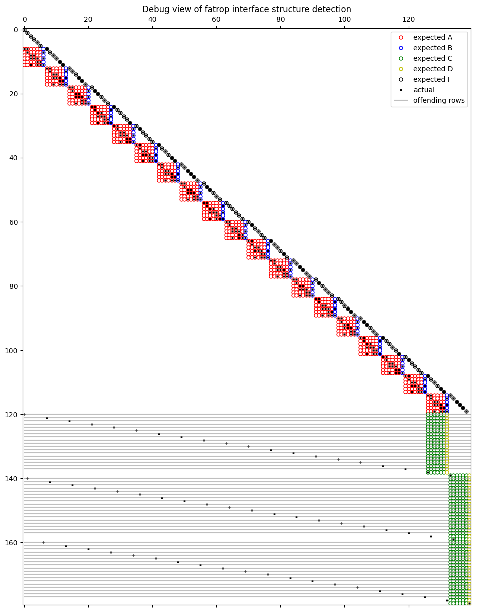
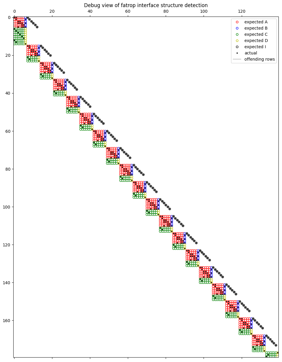
After the data was gathered, we discovered a new solver called FATROP from TU Levin that was just recently interfaced with CasADi. Designed specifically for solving OCPs, it more effectively exploits the banded sparsity structure of the constraint jacobian, allowing for much faster linear solves. We rearranged our variables and constraints to match the structure FATROP expected; see the quadruple-banded structure on the left compared to the single band on the right.
 |
 |
|---|
After doing this, we acheived 5 to 7 times faster solve times compared to IPOPT with MA27, in the ~1ms range.
The other option we tried was Embotech's FORCES Pro, which generates a self-contained solver binary meant for embedded systems. We had great success, with average solve times around half that of FATROP with much lower peaks. This improved performance in some places, but not in a revolutionary manner, so we stuck with the previous solution in an attempt to keep the software stack entirely open source.
Simulation
To evaluate our controller, we built a simulator that mimicked reality as closely as possible. It runs the controller in real-time, timing the runtime and running the simulation for that amount of time before applying the input. It also adds an additional delay to mimic communication latency and adds gaussian sensor noise to all states. The values of these perturbations are as follows.
| parameter | value | unit |
|---|---|---|
| extra latency | ms | |
| m, m/s | ||
| rad, rad/s |
The angular noise values are taken from the encoder datasheet, and the linear noise is estimated from the flexibility of the belt and motor system. The latency is a very conservative estimate intended as a worst-case scenario.
Note that while there is no explicit model mismatch, the use of Euler's method for integration within the controller will introduce enough to be realistic.
Swing-up Trajectory Planning
The swing-up task is effectively modeled as a constrained finite-time optimal control problem (CFTOCP). The MPC controller is meant to solve an approximation of this, but because of how we designed our terminal cost, it does not effectively approximate the true nonlinear cost to go. Therefore, we need to give the MPC controller some additional help for it to complete a swing-up maneuver. This help comes in the form of a pre-planned target trajectory that is known to be feasible.
The math for the terminal constraint will no longer work, so during swing-up, no terminal set is applied. In theory, a terminal set could be designed based on a linearization of the system of deviations, but the time-varying nature of this system means that even if we perform the Lyapunov function-based method described earlier, we cannot show stability, since for time-varying systems it is not sufficient to show
The terminal cost is similarly limited. Thus, these preliminary results simply have the terminal cost computed for the final target state. This qualitatively did not seem to cause many problems.
For each point along path:
- define
- linearize and discretize
- compute DARE solution
- compute
- compute
- solve the optimization to find max terminal cost
- set max terminal cost as a constraint
Results
We evaluated our controller on both the swing-up and stabilizing tasks in the real-time simulator and on hardware. We ran the following three swing up maneuvers:
| Number | ||
|---|---|---|
| 1 | ||
| 2 | ||
| 3 |
And used the following parameters:
- initial state
- state cost matrix
- control cost matrix
The constraints were derived from the limits of the hardware setup.
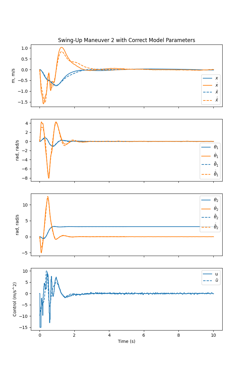
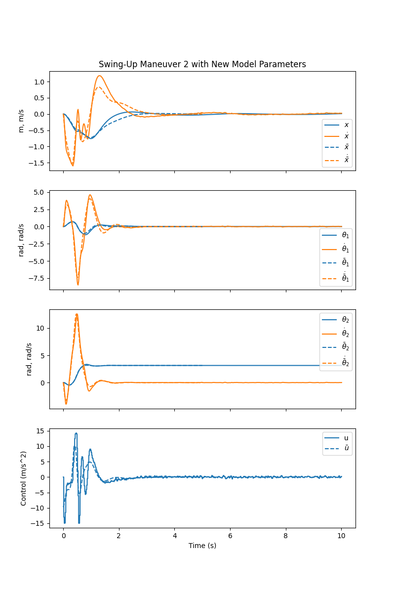
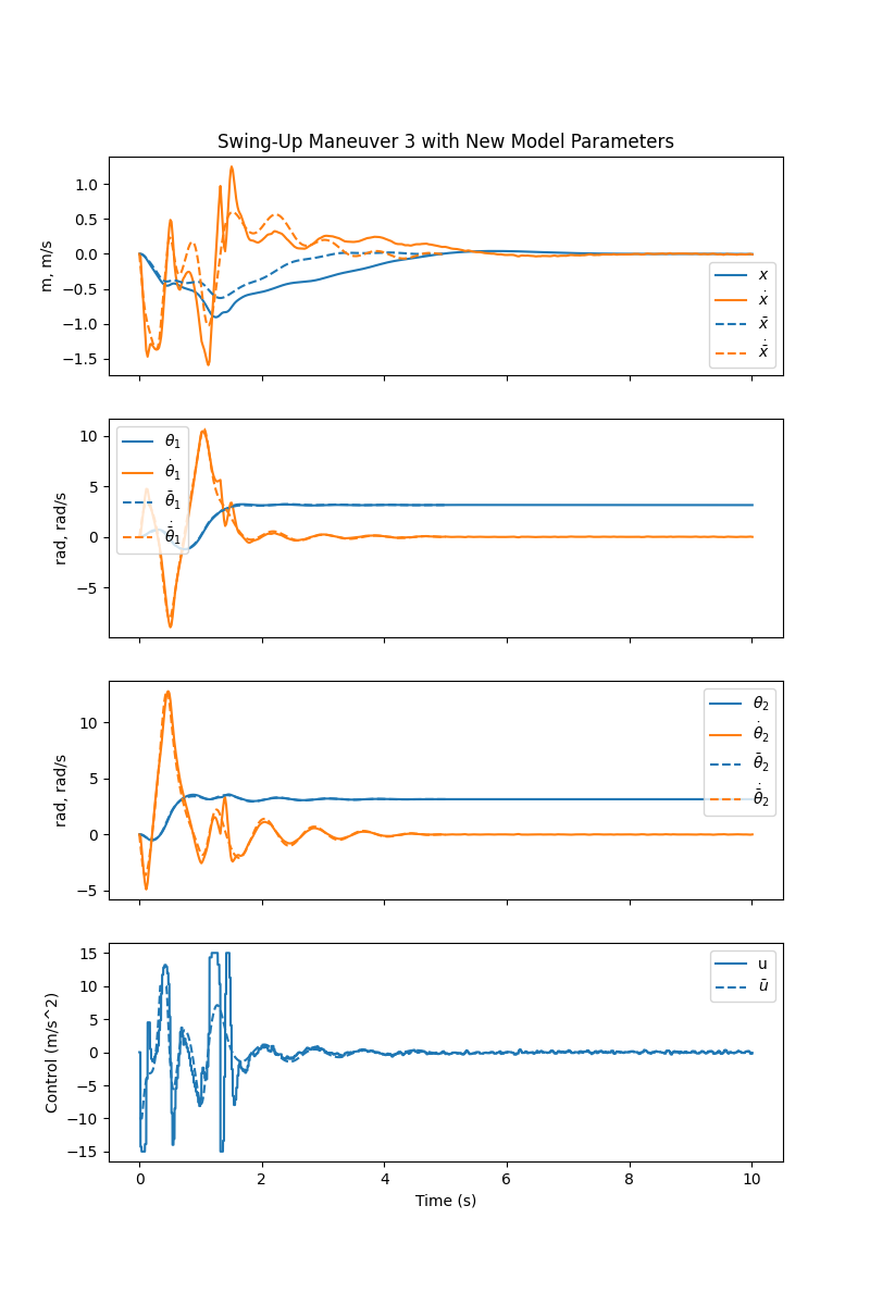
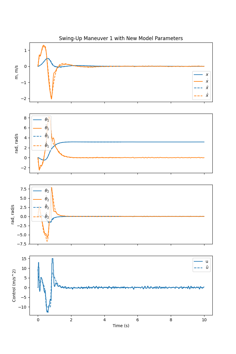
For each maneuver, we ran the simulation once with the same model parameters for MPC, the trajectory planner, and the simulator. We then ran it again with a new set of parameters for MPC and the simulator without recomputing the target trajectories, to test how our controller would perform if the target trajectory was not actually feasible. This introduced more deviation from the trajectory, but all three maneuvers were still reliably completed.


We attempted to run these swing-up maneuvers on the hardware, but they failed. Here is an example of the data collected during a run on the hardware:
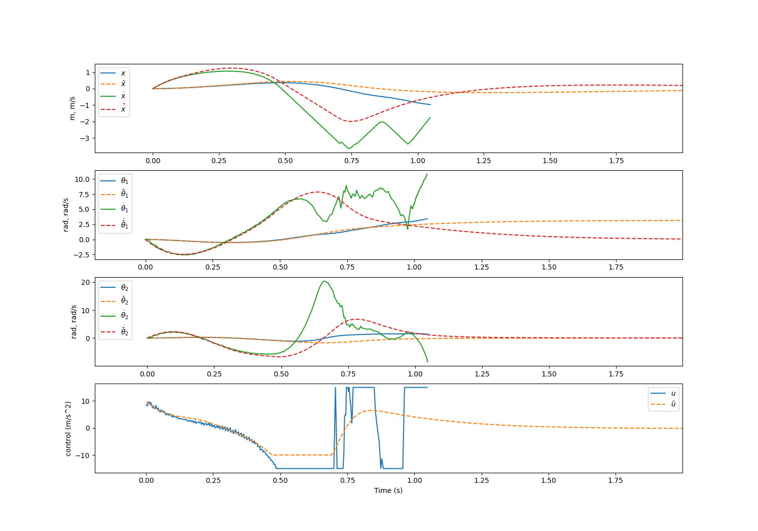
Tracking works well for the first nearly half second, but then it falls apart. This indicates that the model is only good near the origin, and more generally that our system characterization was limiting our performance. Future work could include both better parameter fitting and/or an additional observer to correct for model mismatch.
One factor that made model fitting difficult was the nonlinearity of the encoders, which may be up to
We did, however, find success in the stabilizing tasks on the hardware, producing these results:
On the whole, these results are very good, and serve to validate the simulated results - the amount of oscillation is on the same order of magnitude as in the simulator, and the controller was able to stabilize the system around all equilibrium points.
Conclusions
We have successfully implemented a receding horizon controller which is capable of swinging up and stabilizing a double-inverted pendulum on a cart. We derive the system dynamics using Lagrangian mechanics, which we then use to design a nonlinear model-predictive controller with quadratic stage and terminal costs, the latter derived from the infinite-horizon LQR. We derive a terminal constraint set for this controller that would force recursive feasibility if the system were linear but ultimately conclude that this set is far too small to be practical. Instead, we solve the full CFTOC problem offline to provide a motion plan which our MPC can track with a reasonably sized time horizon. We implement this using CasADi and evaluate it in a SITL (simulator in the loop) environment with additional stresses including latency and noise, where we see very reliable performance. We also test it on a physical test system, where we reliably achieve stabilization, but fail to perform swing-up due to significant model mismatch. We find it likely that the model is only accurate in linearization. From the testing, we draw two main conclusions: first, the factor that most impacts stability is latency. This is not accounted for by the controller, so we are forced to simplify the problem and optimize the code to minimize runtime at all costs. Second, we find that the terminal constraint, although mathematically convenient, proves limiting and impractical.
There is still significant work to be done on this project; further investigations could include better time-varying terminal costs, compensation for constant offsets, investigation of recursive feasibility (or the lack thereof) for controllers with no terminal constraint, or more efficient methods for solving the swing-up motion planning problem.
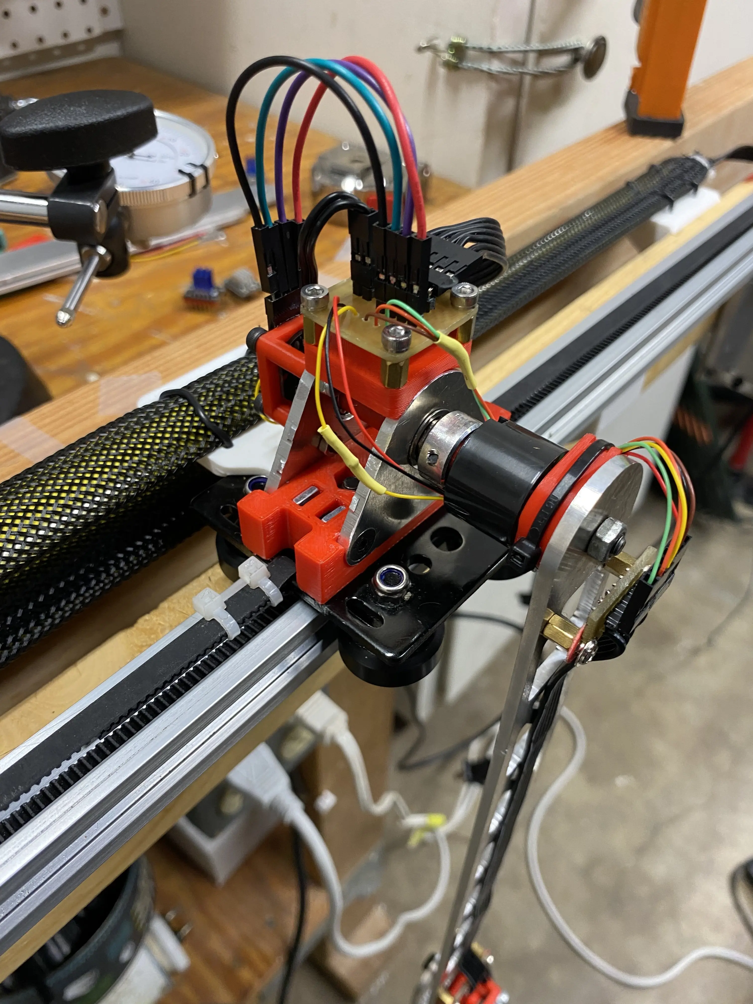
Appendix: Hardware Changes
The hardware was changed significantly from that of the single pendulum. Here is a brief summary of the changes.
- the motor was swapped for a larger Nema 23 size stepper motor
- the motor driver was changed from the A4988 (step/dir control) to the TMC2208 (allows setting velocity over UART) then finally to the TMC5160 (allows setting acceleration over SPI). Removing the reliance on a custom-built ramp generator saved significant time and effort.
- the motor power supply was increased from 12v to 48v (no longer limited by the stepper driver)
- the pulley size was increased to 80T
- the pendulums were redesigned to be lightweight and precise
- aggressive pocketing
- pivots were redesigned to reduce friction and slop
- encoder mounts were redesigned to borrow precision from the CNC to ensure alignment of the encoder and the axis
- the wire management was improved:
- drag chain for cart movement
- custom PCBs on the cart and first pendulum to keep wires tidy and handle the SPI daisy-chaining
- proper connectors crimped everywhere
- the encoders were changed from AS5600 (12 bit, I2C) to AS5048 (14 bit, SPI). This did not significantly increase precision due to the noise level of the AS5048, but using the SPI protocol allowed for much faster polling frequencies.
- the microcontroller was swapped from the RP2040 to the Teensy4.0, which is much faster (600Mhz) and has an FPU for high speed float math.
- the serial protocol was redesigned to send raw binary instead of ASCII, reducing latency.